Edge Path Bundling

Overview

This is the comprehensive code documentation for the Edge Path Bundling project, which implements the edge bundling algorithm described in "Edge-Path Bundling: A Less Ambiguous Edge Bundling Approach" by Wallinger et al. (2021). Our implementation provides a complete Python framework for graph visualization with edge bundling capabilities, featuring interactive exploration tools and multi-dataset support.

EPB addresses the critical challenge of visual clutter in network visualizations by grouping related edges into smooth, bundled paths while preserving the underlying network structure. Unlike traditional edge bundling approaches that can introduce visual ambiguity, this implementation maintains topological correctness through careful path selection and distortion control.

Project Structure

The project follows a modular architecture with clear separation of concerns across four main packages:

Core Algorithm (src/core/) - Implementation of the edge path bundling algorithm with spatial distance calculations
Data Loading (src/data_loader/) - Specialized loaders for different network dataset formats
Visualization Engine (src/visualization/) - Plotly-based rendering with Bézier curve generation and multi-dimensional support
Interactive Dashboard (src/dashboard/) - Web-based interface for parameter exploration and real-time visualization

Folder	File	Description
src/core	__init__.py	Package initialization
src/core	bundling.py	Core edge bundling algorithm implementation
src/data_loader	__init__.py	Package initialization
	air_traffic.py	OpenFlights airport and route data loader
	brain_connectivity.py	Brain connectivity GraphML data loader
	migration.py	US county migration flows data loader
src/visualization	__init__.py	Package initialization
	curves.py	Bézier curve generation and path smoothing utilities
	plotly_renderer.py	Plotly-based network visualization renderer
src/dashboard	app.py	Interactive Dash web application
src/dashboard	static/	Static assets (logos, CSS)

bundling.py - Core Algorithm Implementation

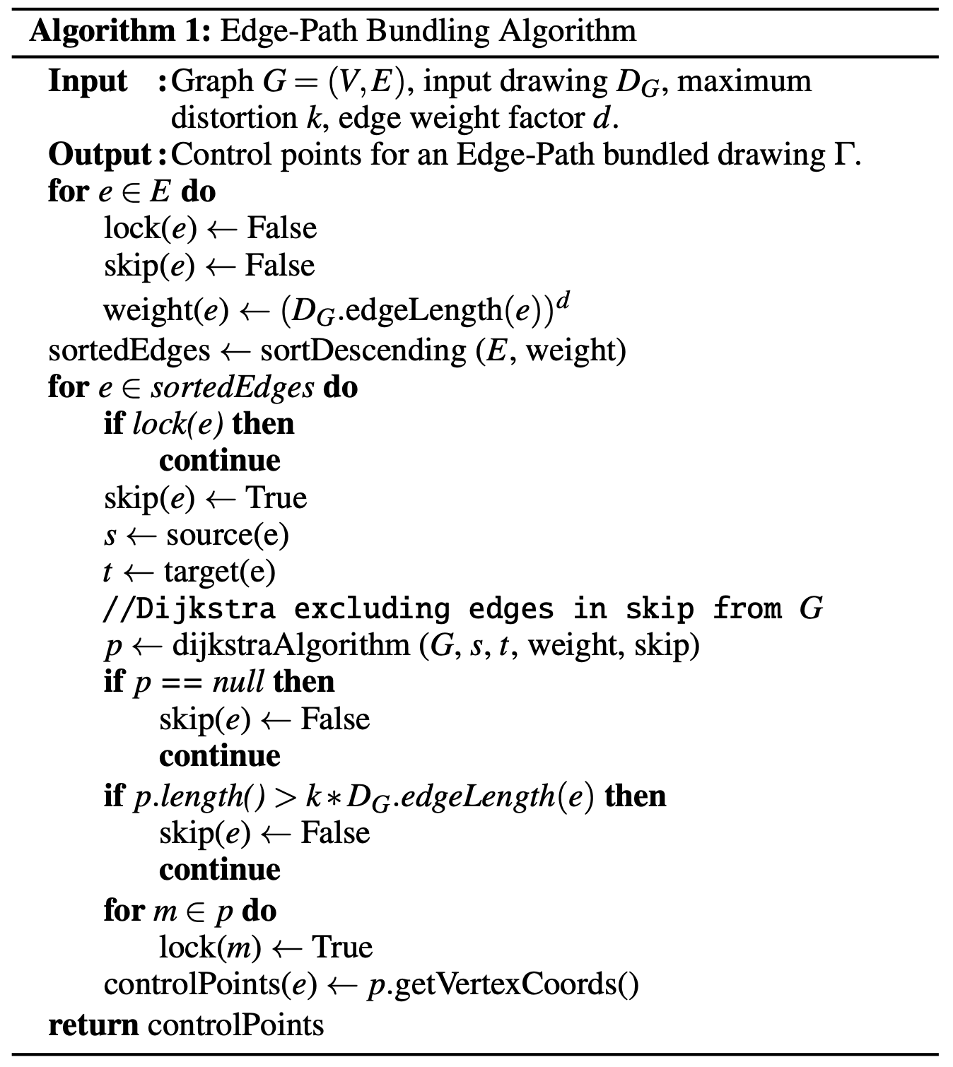
This module contains the heart of our edge path bundling system, implementing Algorithm 1 from Wallinger et al.'s paper with additional optimizations for real-world graph processing. The implementation carefully balances computational efficiency with visual quality, providing robust handling of diverse network topologies and coordinate systems.

Edge Path Bundling Algorithm Overview

The core algorithm processes edges in weight-descending order, attempting to route each edge through existing bundled paths while respecting a maximum distortion threshold k. The approach ensures that bundled paths remain meaningful representations of the underlying network topology.

The following image shows the EPB algorithm that Wallinger et. al. proposed in their paper. The implementation was close to straight forward with adding some helper functions for a cleaner code.

Algorithm 1 — Edge-Path Bundling Algorithm proposed by Wallinger et. al..

Core Functions

create_graph(nodes: List[Dict], edges: List[Tuple], distance_type: str) → nx.DiGraph

Graph construction utility that builds NetworkX graphs from raw coordinate data.

Supports both 2D and 3D coordinate systems
Automatically calculates spatial edge weights using specified distance metric
Handles missing or invalid coordinate data gracefully
Preserves original node metadata for visualization purposes

bundle_edges(graph: nx.DiGraph, k: float, d: float) → Dict

Main algorithm orchestrator that implements the complete edge path bundling workflow.

Input: NetworkX directed graph with spatial node coordinates
Parameters: k (distortion threshold), d (edge weight exponent)
Returns: Dictionary mapping original edges to bundled path sequences

Although this algorithm treates k and d as floats they should not be any number. Since d is a factor it makes sense to treat it as integer. Through the experiments that were conducted in the original paper d should be in the set {1,2,3}. A maximum distortion factor k above 3 does not change the outcome much. Our interactive dashboard takes those observations into account, therefore both only range from 1 till 3 with k also considering decimal numbers.

Distance Calculation Functions

haversine_distance(lat1, lon1, lat2, lon2) → float

Great circle distance calculation for geographic coordinates using the Haversine formula.

distance = 2R × arcsin(√(sin²(Δφ/2) + cos φ₁ × cos φ₂ × sin²(Δλ/2)))

Used for any lat/lon coordinate systems. In our case air traffic and migration networks. The radius R is for us the radius of the earth 6371.0km.

euclidean_distance(x1, y1, x2, y2, z1=None, z2=None) → float

Euclidean distance in 2D or 3D space with optional z-coordinate support. Following formular shows how to compute the euclidean distance between three dimensional nodes.

    distance =√((x₂ − x₁)²+ (y₂ − y₁)²+ (z₂ − z₁)²)

Pathfinding Implementation

dijkstra_with_skip(graph, source, target, locked_edges) → List

Modified Dijkstra's algorithm that respects edge locking for bundle construction.

Excludes previously locked edges from path consideration
Returns shortest available path or None if no valid path exists
Optimized for repeated calls on dynamically changing edge availability
Maintains NetworkX compatibility for easy integration

data_loader

Collection of specialized data loading modules that handle different dataset formats and coordinate systems. Each loader creates NetworkX graphs with appropriate distance metrics and spatial attributes for the bundling algorithm.

air_traffic.py

Loads OpenFlights airport and route data, handling CSV parsing for airport coordinates and route connections. Uses haversine distance for geographic calculations. Filters invalid entries and creates directed graph with airport metadata including IATA codes, cities, and coordinates.

brain_connectivity.py

Processes GraphML files from the Human Connectome Project containing 3D brain region coordinates and structural connections. Handles MNI coordinate system conversion and creates 3D visualizations using Euclidean distance. Supports filtering by connection strength thresholds.

migration.py

Parses US Census Bureau county-to-county migration flow data. Converts FIPS county codes to geographic coordinates and filters by minimum flow thresholds. Uses haversine distance for geographic calculations and handles coordinate lookup for US counties.

plotly_renderer.py

Comprehensive visualization module that renders bundled graphs using Plotly with support for 2D geographic maps, 3D brain visualizations, and smooth Bèzier curve generation.

Visualization Types

Geographic Maps - Uses Plotly's Scattergeo for air traffic and migration data with automatic US/world map detection
3D Brain Visualization - Interactive 3D plots for brain connectivity data with rotation and zoom controls
Standard Network Plots - 2D scatter plots for general network data with optional geographic overlays

Curve Generation

Implements smooth Bèzier curve generation using recursive subdivision and De Casteljau's algorithm. Supports configurable smoothing levels (adding control points) and sampling resolution. Works in both 2D and 3D coordinate systems for consistent curve appearance.

curves.py - Bézier Curve Generation

Dedicated module for smooth curve generation following the paper's approach to path visualization. Implements advanced Bézier curve mathematics with recursive smoothing algorithms to create visually appealing bundled edge representations while maintaining mathematical precision.

A Bézier curve is a type of parametric smooth curve defined by a set of control points P₀, P₁, ..., Pₙ.

B(t) = Σᵢ₌₀ⁿ (n choose i) × (1-t)ⁿ⁻ⁱ × tⁱ × Pᵢ

Where t ∈ [0,1] parameterizes the curve from start to end.

Bezier curve — Cubic Bèzier curve with four control points.

Curve Generation Pipeline

Control Point Extraction: Extract spatial coordinates from bundled path nodes
Recursive Smoothing: Apply iterative midpoint insertion for smoother curves
Bézier Interpolation: Generate smooth curves using De Casteljau's algorithm
Adaptive Sampling: Create optimal point density for rendering

Core Functions

generate_control_points(path_nodes, node_positions, smoothing_level=2) → List[np.ndarray]

Control point generator that converts bundled paths into smooth curve control points.

Input: Node sequence from bundled path, coordinate mapping
Process: Extracts coordinates and applies recursive smoothing
Returns: Array of control points suitable for Bézier interpolation

apply_recursive_smoothing(points, smoothing_level) → List[np.ndarray]

Recursive smoothing algorithm implementing the paper's approach for curve refinement.

Iteratively inserts midpoints between existing control points
Each iteration doubles the control point density
Maintains curve continuity while increasing smoothness
Configurable smoothing levels for different quality requirements

generate_bezier_curve(control_points, num_samples=100) → np.ndarray

Bézier curve interpolation using De Casteljau's algorithm for numerical stability.

Supports arbitrary-degree Bézier curves based on control point count
Configurable sampling density for different rendering requirements
Handles both 2D and 3D coordinate systems seamlessly
Optimized for real-time interactive applications

bezier_point(control_points, t) → np.ndarray

Single point evaluation on Bézier curve using De Casteljau's algorithm.

Numerically stable recursive evaluation
Handles edge cases (t=0, t=1) correctly
Linear time complexity O(n) for n control points
Used internally by curve sampling functions

3D Curve Support

generate_3d_control_points(path_nodes, node_positions, smoothing_level=2) → List[np.ndarray]

3D curve generation specifically designed for brain connectivity visualization.

Handles x, y, z coordinate extraction from 3D node positions
Maintains spatial relationships in 3D space
Compatible with MNI coordinate systems used in neuroimaging
Supports interactive 3D visualization with Plotly

One note to add is that higher smoothing levels and sample counts improve visual quality but increase computational cost which is problematic for real-time viusalizations. A recommended setting would be smoothing_level=2, num_samples=80 for good balance of quality and performance. Also the original paper sticked to 2 for the smoothing parameter, however, we wanted the user to experience the differences it can make.

app.py

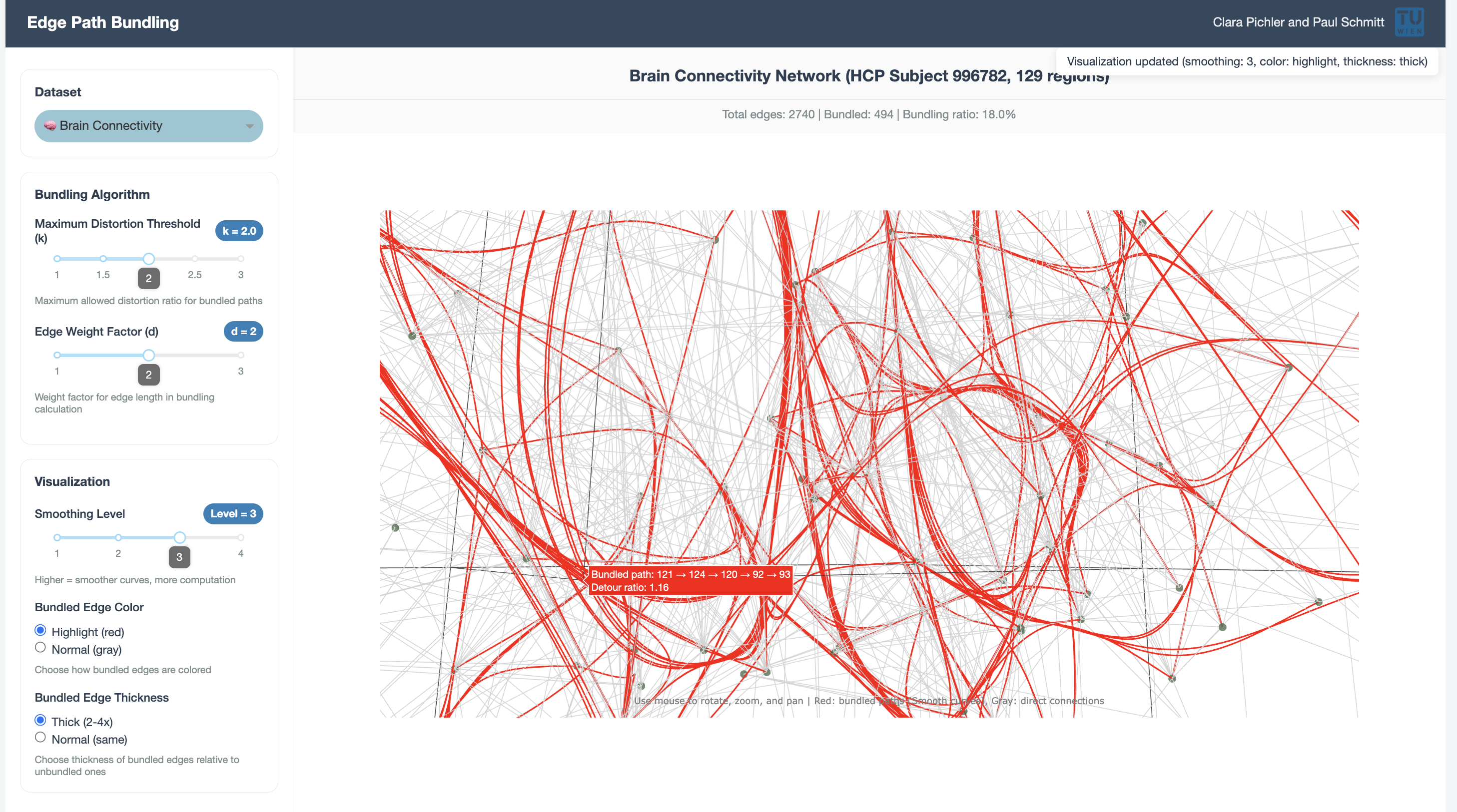
Interactive Dash web application that provides a user interface for exploring edge path bundling on different datasets. Features parameter controls and real-time visualization updates.

Key Features

Parameter Controls - Sliders for maximum distortion threshold (k) and edge weight factor (d).
Dataset Selection - Dropdown for switching between brain, air traffic, and migration datasets.
Visualization Options - Slider for smoothing parameter for the Bèzier curves as well as options to highlight bundled edges either through color or thickness.
Statistics - Number of edges of the selected network, number of bundled edges and percentage of how many edges were bundled. Also when hovering over a bundled edge the detour ratio as well as its control points become visible.

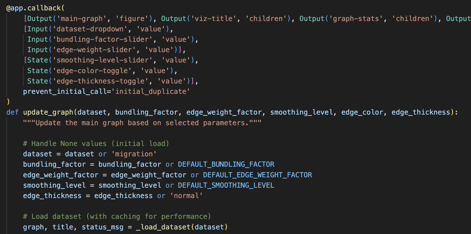
Callback Architecture

Uses Dash callbacks for reactive updates: parameter displays update immediately, dataset changes reset controls, bundling recalculation occurs for algorithm parameters, and updates for visualization-only changes.

Performance Constants

Since the algorithm takes some time due to the frequent calling of the Dijkstra's algorithm as well as does the visualization take some time with a high smoothing parameter, we needed to add some limitations on the data.

Major airports limited to 50
Migration data filtered to top 100 counties
Minimum flow threshold of 3,000 for migration data
Fixed curve sampling at 80 points for smooth rendering